 menu
menu
Determining the link budget is a vital step in every satellite mission. Its purpose is to determine whether satellite and ground station communication configurations are able to transmit and receive the necessary volume and quality of data to ensure the mission objectives are met. This process entails determining the associated gains and losses that define the system, calculating the received power, comparing the received signal to ambient noise, and ultimately determining the amount of useful data that can be read.
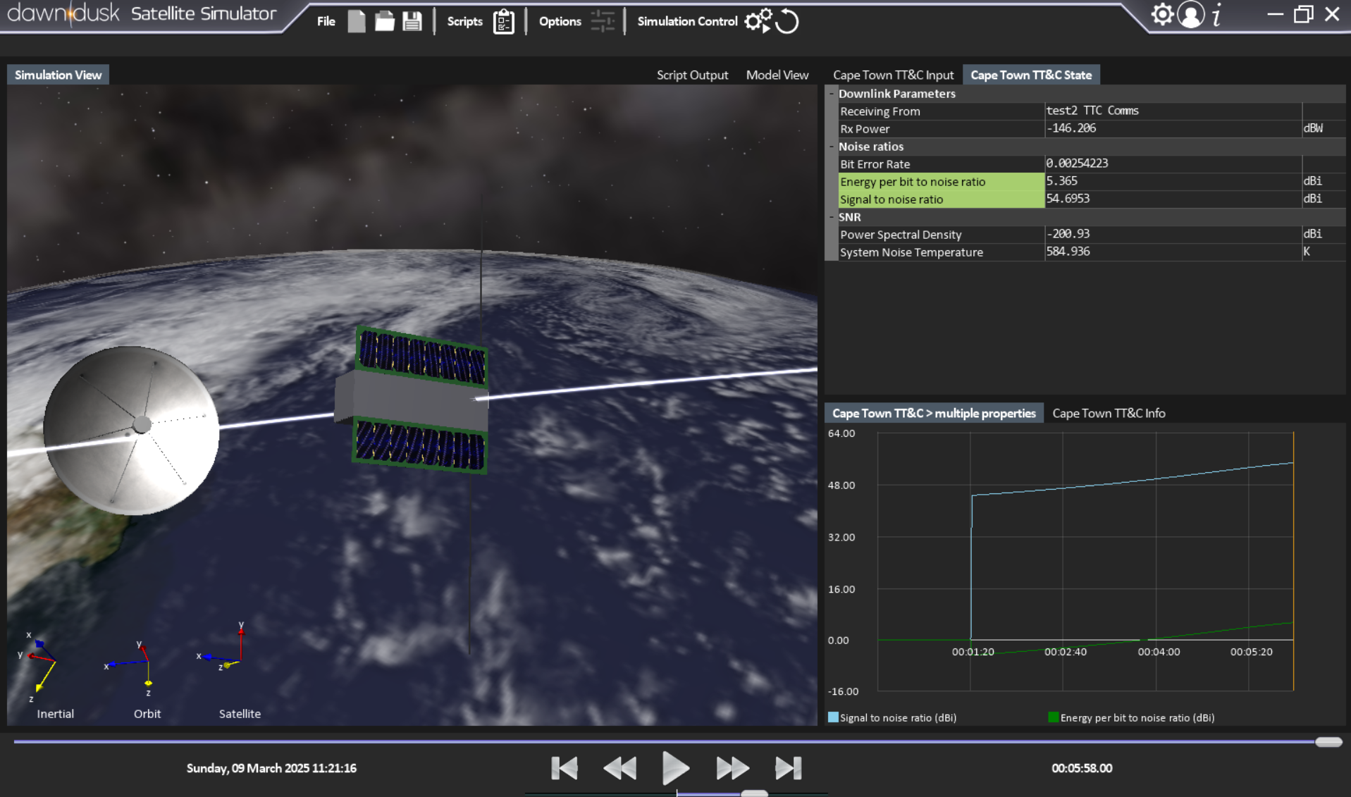 Figure 1: A satellite performing a data downlink over a Cape Town ground station.
There are many tools to achieve this depending on the stage of mission development. Techniques range from back-of-pamphlet calculations to dedicated software suites. As D2S2 primarily remains an orbital dynamics simulation, it is recommended that the link-budgeting functionality only be used for early- to mid-development analyses. Nevertheless, D2S2 offers competitive advantages to both students and professional developers:
Table 1: Competitive advantages offered by D2S2 for both student and professional users
| Free features | Licensed features |
|---|---|
| Easy scenario / test setup | Constellation simulation |
| Dynamic multi-orbit simulation | Multi-ground station simulation |
| Satellite attitude simulation | Scripted user tests |
| Link & power budget simultaneous simulation | User defined radiation patterns |
| Easy data extraction | Modularity to simulate the user's required accuracy |
| User-defined modulation schemes |
To reduce user uncertainty regarding the link budget functionality, this page is dedicated to explaining how D2S2 performs the tests, what input parameters are required from the user, and what benchmarks were used to validate the functionality.
As the link budget calculation requires multiple input and derived parameters, Table 2 presents a nomenclature used throughout this page.
Table 2: Nomenclature used in the calculation of the link budget
| Symbol | Name | Quick description | Unit |
|---|---|---|---|
| System characteristics | |||
| PTX | Transmitting power | The power pushed to the antenna of the transmitter. | W |
| LI | Insertion loss | The loss applied to the signal between the transceiver and the antenna due to internal circuity. Often merged with LL. | dBi |
| LL | Line loss | The loss applied to the signal between the transceiver and antenna due to cabling. Often merged with LI. | dBi |
| GTX | Transmitting Gain | Gain applied to the signal before reaching the antenna. | dBi |
| GA | Antenna Gain | Gain applied to the signal by the antenna. Different values for TX and RX are common. | dBi |
| LP | Pointing loss | Losses applied to the signal due to antenna misalignment. This is heavily dependent on the antenna's radiation pattern. | dBi |
| LFS | Free space loss | Losses applied to the signal due to it traveling through space. | dBi |
| LP | Polarity loss | Losses applied to the signal due to non-perfect carrier electromagnetic fields. | dBi |
| Latm | Atmospheric loss | Losses applied to the signal due to traveling through the atmosphere. | dBi |
| LM | Modulation loss | Losses applied to the signal due to the implemented modulation scheme. | dBi |
| Rb | Bit rate | The rate at which bits are carried in the transmitted signal. | bits/s |
| Limp | Implementation losses | Losses applied to the signal due to the distortion of intermodulation, phase noise, and other practicalities of real transmitters. | K |
| Noise parameters | |||
| TA | Antenna noise temperature | The noise temperature emitted by the receiving antenna. | K |
| TC | Circuit noise temperature | The noise temperature emitted by the internal receiver circuitry. | K |
| Frec | Noise factor | The noise factor (at 290K) | |
| Derived parameters | |||
| Tsys | System noise temperature | The ambient system noise is calculated as a summation of other noise factors. | K |
| Co | Received system power | The power received by the transceiver after all gains and losses are accounted for | dBW |
| N0 | Power spectral density | The ambient noise power with which the received signal must contend with to be read. | dBi |
| BER | Bit error rate | The ratio of bits that become corrupted and consequently need to be resent. | |
| EIRP | Equivalent Isotropic Radiative Power | The actual signal power just after exiting the transmitter system, but before accounting for the losses associated with traveling through space. | dBW |
Link budgets are most conveniently done as the summation of gains and losses (in dB) experienced by a transmitted signal as it travels from the transmitter to the receiver. Consider Figure 1 below, which presents the overview diagram of the components, gains, and losses typically found in a link budget calculation. This section will present the calculations required to determine the major outputs of a link budget as the signal is generated at the transmitter, travels through the atmosphere, and gets received by the receiver.
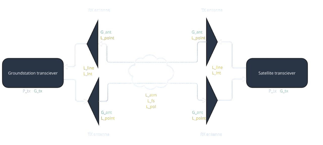 Figure 2: Overview of link budget setup, standard gains, and standard losses.
As mentioned previously, the link budget is most easily done by utilizing decibel units in the summation of the gains and losses. For a parameter P with the unit [U], the decibel presentation P[dBU] is calculated as in Equation 1:
| \(P[dBU] = 10log_{10}(P[U])\) | [1] |
The calculation of the Received Signal Power (Co) considers all the gains and losses between the transmitter and receiver. The relevant derived parameters are presented in Equations 2 - 4 and the received signal power is presented in Equation 5:
The Equivalent Isotropic Radiative Power (EIRP) presents the power of the transmitted signal just after leaving the transmitter antenna, but before the losses of propagation through space are applied. Equation 2 presents how this parameter is calculated:
| \(EIRP = P_{Tx}G_{Tx}(\frac{1}{L_{Tx}})\) | [2] |
| where, | |
| \(L_{Tx} = L_{I-Tx}*L_{L-Tx} * L_{P-Tx}\) | (Losses at emission) |
The gains and losses associated with the receiving system are applied in the same way barring the initial signal power.
As the signal travels, it experiences free space loss (LFS) as well as propagation loss (Lprop). These two parameters are presented in Equation 3 and Equation 4.
| \(L_{FS} = (\frac{4 \pi R}{\lambda})^2\) | [3] |
| where, | |
| \(\lambda\) = carrier wavelength (m), | |
| R = distance from the emitter (m) | |
| \(L_{prop} = L_{atm} * L_{P}\) | [4] |
Calculating the received power is the summation of the values above. This calculation is presented in Equation 5.
| \(C_{o} = [EIRP] * [\frac{1}{L_{FS}} * \frac{1}{L_{prop}}] * [G_{A-Rx} * \frac{1}{L_{Rx}}]\) | |
| \(C_{o} = [P_{Tx}G_{Tx}(\frac{1}{L_{Tx})}] * [(\frac{\lambda}{4 \pi R})^2 (\frac{1}{L_{prop}})] * [G_{A-Rx} (\frac{1}{L_{Rx}})]\) | [5] |
The next important derived parameter is the Signal to Noise Ratio (\(\frac{C_o}{N_0}\)) of the received signal. This ratio represents how strong the signal is when compared to the ambient noise around the receiver. The signal-to-noise ratio is presented in Equation 6 and expanded in Equation 7.
| \(\frac{C_o}{N_0} = \frac{C_o}{k T_{sys}}\) | [6] |
| where, | |
| \(N_o = k T_{sys}\), | Spectral noise density |
| \(k = 1.38E^{23}\), (J/K) | Boltzmann constant |
| \(T_{sys} = \frac{T_{ant-Rx}}{L_{I-Rx}} + \frac{L_{I-Rx}-1}{L_{I-Rx}}*T_{cir-Rx} +T_{rec}\), | System noise temperature |
| \(T_{rec} = (F_{rec}-1)T_0\), | |
| \(T_0 = 290\), (K) | |
| and thus, | |
| \(\frac{C_o}{N_0} =[P_{Tx}G_{Tx}(\frac{1}{L_{Tx})}] * [(\frac{\lambda}{4 \pi R})^2 (\frac{1}{L_{prop}})] * [ \frac{G_{A-Rx}}{kT_{sys}} (\frac{1}{L_{Rx}})]\) | [7] |
Additionally, there are further losses associated with the modulation scheme (\(L_{mod}\)) as well as other implementation losses (\(L_{imp}\)). It is then useful to consider the Energy per Bit to Noise Ratio (\(\frac{E_b}{N_o}\)) to determine the probable success rate of intercepting and interpreting each bit. This ratio is presented in Equation 8 and expanded in Equation 9.
| \(\frac{E_b}{N_o} = \frac{1}{L_{imp}}*\frac{1}{L_{mod}}*\frac{(\frac{C_o}{R_b})}{N_0}\) | [8] |
| and thus, | |
| \(\frac{E_o}{N_0} =[ \frac{1}{L_{imp}}*\frac{1}{L_{mod}}] * [\frac{P_{Tx}G_{Tx}(\frac{1}{L_{Tx})}}{R_b}] * [(\frac{\lambda}{4 \pi R})^2 (\frac{1}{L_{prop}})] * [ \frac{G_{A-Rx}}{kT_{sys}} (\frac{1}{L_{Rx}})]\) | [9] |
The Bit Error Rate is the rate at which bits in the carrier signal will be misread or lost due to the ambient noise around the receiver. This value is most often a function of the Energy per Bit to Noise Ratio and the modulation scheme chosen. For example, the BER for BPSK and QPSK modulation is expressed in Equation 9.
| \(BER = \frac{1}{2} * erfc(\sqrt{\frac{E_b}{N_o}})\) | [9] |
It can be noted, however, that these equations can become involved and difficult to compute within a simulated environment. The differing method in which D2S2 (and other simulators) determines the BER is presented in the sections below section.
As mentioned previously, D2S2 is primarily an orbital dynamics simulator, and as such the process and inputs to do link budget analyses may not be immediately clear to new users. In addition, some features may be more or less developed than other link-budget calculators to better utilize the strengths of the program. As such this section will present instructions and explain the various parameters required.
D2S2 scenarios consist of a number of models that make up the satellite and ground station components. Instead of presenting all link budget parameters in a calculator tool, D2S2 rather requires that these parameters be given as model inputs and states. The two important models required for a link budget the:
Both of which will be loaded into the scenario after completing Tutorial 2. An overview of how these two models interact is presented in Figure 3. Following the signal path in this figure reveals differences in parameter definition and utilization during uplink and downlink. Many of these changes are purely definitional (for example merging some losses) while others are operational to the D2S2 environment. In the following subsections, these functional changes will be discussed.
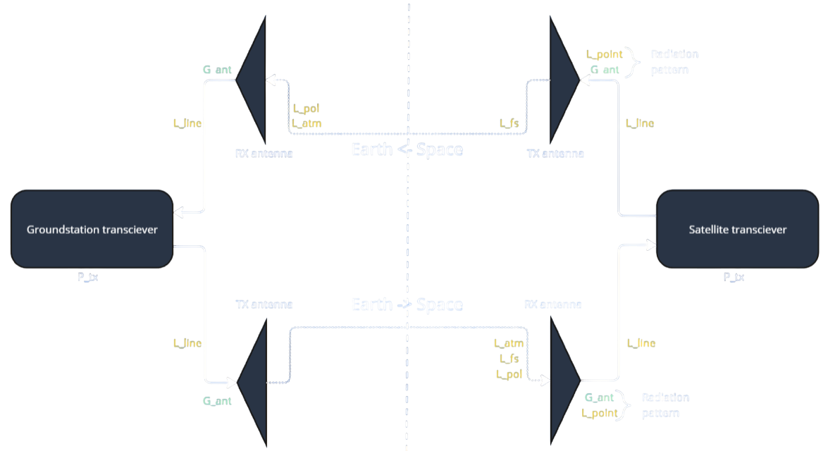 Figure 3: An overview of how the carrier signals are represented during communication between the simulated ground station and satellite transceiver in D2S2.
Consider Figure 4 which presents a code diagram of how D2S2 calculates the received signal power between the models.
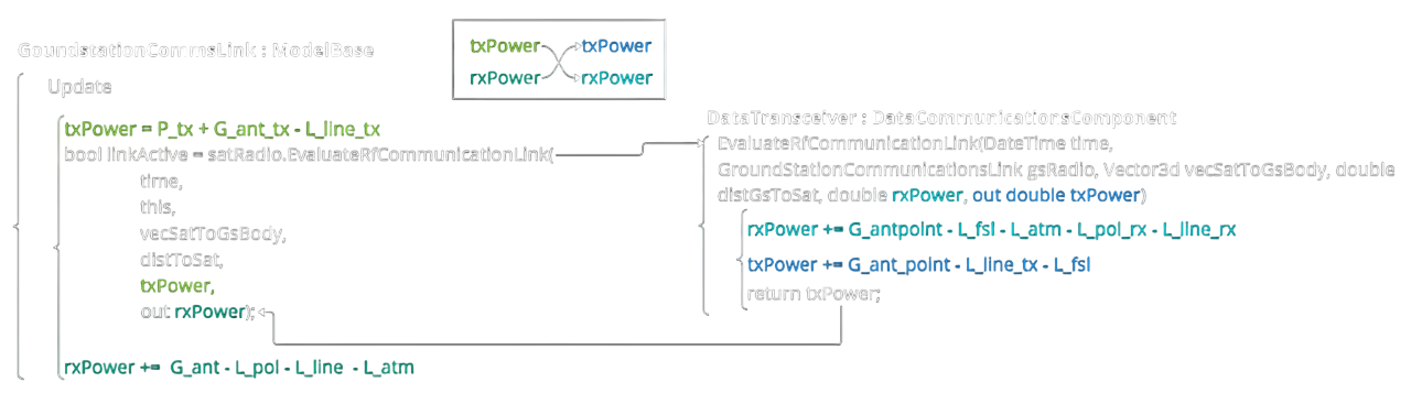 Figure 4: An overview code diagram of the interactions between the D2S2 ground station and satellite transceiver models. In the diagram, how the parameters are summated in the calculation of the received signal is made apparent and can be used to more directly follow the path presented in Figure 3. Critically, note that all parameters are expressed in decibel format.
Critically, there are a number of limitations and design choices that should be considered by the user when performing a link budget analysis. These are as follows:
Satellite transceiver
Ground station
As can be deduced when considering the effect of these changes, the accuracy of the link budget analysis is not diminished should the user accommodate the specific parameter definitions.
The Signal to Noise Ratio (\(\frac{C_o}{N_o}\)) and Energy per Bit to Noise Ratio (\(\frac{E_b}{N_o}\)) remain operationally exactly the same as described in the previous section. All the noise temperature parameters are obtained as inputs from the user and as such no changes are made to the mathematical theorem. This functionality is currently, however, only implemented for signals in the space->Earth direction of travel due to the dynamic wild nature of LEO noise temperature patterns.
As mentioned previously, the equations relating the Bit Error Rate (\(BER\)) to the Energy per Bit to Noise Ratio ( \(\frac{E_b}{N_o}\) ) are involved calculations and difficult to implement in a simulated environment. To overcome this, D2S2 captures four points of measured data for some of the major modulation schemes:
Through these points, logarithmic regression can be applied to capture the parameters defining the logarithmic function. Through this method, D2S2 can readily approximate the corresponding \(BER\) at simulated \(\frac{E_b}{N_o}\) values. The feature allowing users to add their own modulation schemes is planned to be implemented in the future.
As can be noted above, modelling atmospheric attenuation as a static variable is a simplification that prevents detailed link budget analysis. As these calculations create additional programmatic overhead, its left as a toggleable feature. To enable complex atmospheric modelling, an input must be set in the GroundstationTransceiver model as seen in Figure 5. Note that complex atmospheric loss modelling is only applicable to signals travelling in the space -> Earth direction.
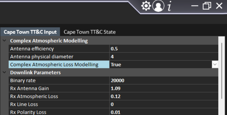 Figure 5: Complex atmospheric loss modelling requires to be enabled an input parameter.
Atmospheric attenuation is the sum of several physical phenomena experienced by a signal as it travels from space through the atmosphere. It is vital to carefully consider each of these phenomena and their effect on the signal as a function of signal frequency, satellite elevation and geographic location. The mathematical definition of atmospheric attenuation as implemented in D2S2 is presented in Eqn 10, similar to as implemented in [1] and [2].
| \(L_{atm} = A_{gas}+\sqrt{(A_{rain} + A_{cloud})^2 + A_{scint}^2}\) | [10] |
This implementation in D2S2 is based on literature made available by the International Telecommunications Union (ITU) and specifically draws from [2 - 8]. Using [2] as a starting point, the user is encouraged to investigate these sources to understand the assumptions and limitations of the simulation.
Attenuation due to scintillation refers to rapid fluctuations in signal amplitude and phase caused by small-scale variations in the refractive index of the propagation medium (in this case the ionosphere and troposphere). This is especially of concern for low satellite elevation angles. The method in which scintillation is modelled can be found in [2, sec 2.4]. Critically, there are a number of limitations and design choices that should be considered by the user when performing a link budget analysis. These are as follows:
Attenuation due to gas is primarily of concern for frequencies larger than 10GHz and can typically be neglected for smaller frequencies. The method in which atmospheric gas attenuation is modelled in D2S2 can be found in [3, Annex 2]. Critically, there are design choices that should be considered by the user when performing a link budget analysis. These are as follows:
Much like attenuation due to gas, attenuation due to clouds, rain and fog is of larger concern to higher frequencies. D2S2 utilises the slant path instantaneous cloud attenuation prediction method as presented in [8] to model this loss.
Attenuation due to rain is currently not implemented in D2S2.
Attenuation due to sand and dust storms is currently not implemented in D2S2.
Benchmark tests is conducted to compare D2S2 link budget results to those generated by other recognized budgeting tools. Primarily, the results are compared to that of RF-Comlink [1] for frequencies within the recommended range. The method by which this is done is to feed RF-Comlink orbital and attitude data taken from D2S2. By extracting the link budget analyses for a time period, a direct comparison with D2S2 can be performed for each timestep. This section presents the results of these analyses.
Figure 6 presents a comparison of the Rx power as generated by RF-Comlink and D2S2 for a single flyby. Also consider Table 3 which presents the average difference of the captured data over the course of 12 hours. The comparison is made over multiple orbits and using different frequencies. What can be seen is that for the majority of frequencies important to LEO satellite communication, the D2S2 simulator performs link budget analyses accurately enough for early- to mid- development. Should there be uncertainty regarding the D2S2 modelling accuracy, clients are encouraged to perform their own comparisons or raise issues to the development team.
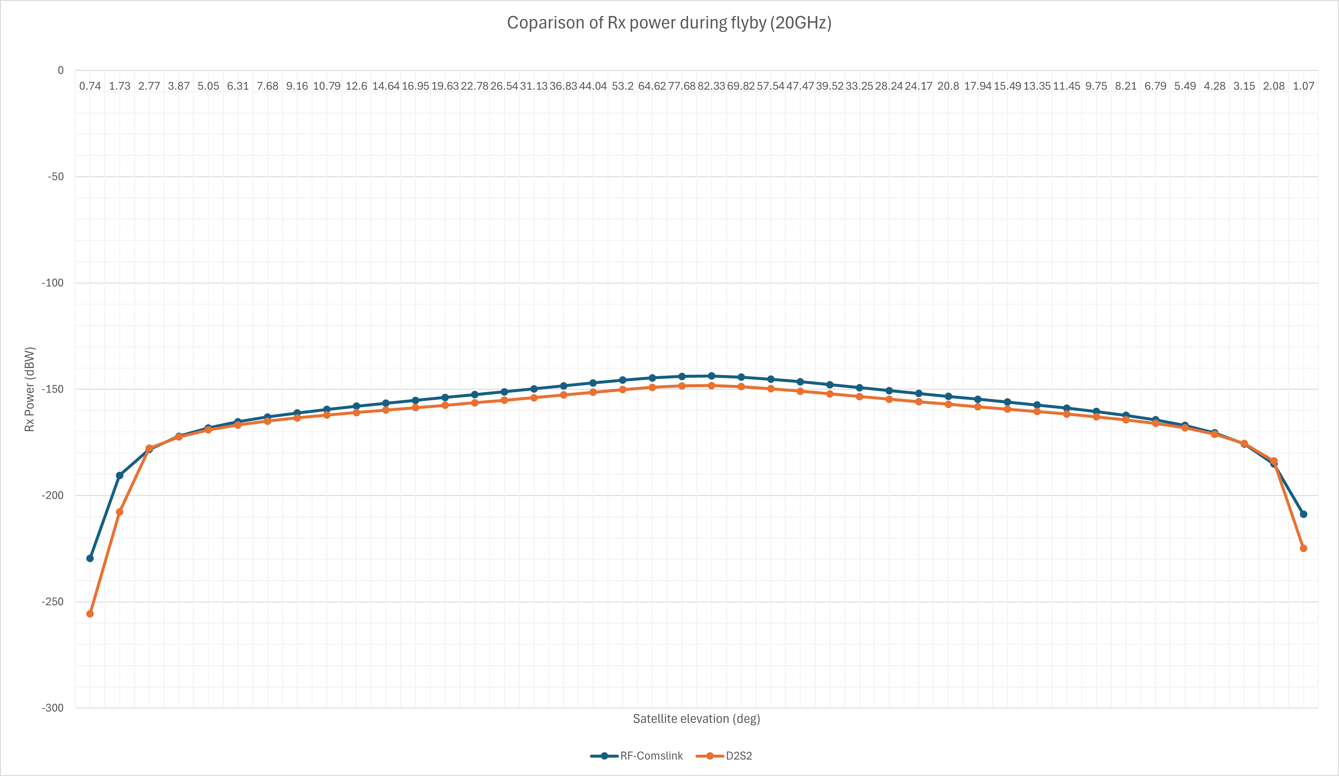 Figure 6: A comparison of Rx-Power of the ground station during a flyby analysed through RF-Comlink and D2S2
Table 3: Comparison of received power as analysed through RF-Comlink and D2S2
| Frequency | Average error (%) | Average error (%) at elevation greater that 5 deg |
|---|---|---|
| 2 GHz | -0.3 | -0.3 |
| 10 GHz | -1.6 | -0.9 |
| 20 GHz | -1.2 | 1.8 |
| ID | Description |
|---|---|
| 1 | H. Guillon, Technical documentation of RF-COMLINK. CNES, Dec. 12, 2022. [Online]. Available: https://www.connectbycnes.fr/en/rf-comlink| |
| 2 | International Telecommunications Union, Propagation data and prediction methods required for the design of Earth-space telecommunication systems, Recommendation ITU-R P.618-14, Aug. 2023. [Online]. Available: https://www.itu.int/rec/R-REC-P.618-14-202308-I/en| |
| 3 | International Telecommunications Union, Attenuation by atmospheric gases, Recommendation ITU-R P.676-10, Sept. 2013. [Online]. Available: https://www.itu.int/rec/R-REC-P.676-10-201309-I/en| |
| 4 | International Telecommunications Union, Reference atmospheres, Recommendation ITU-R P.835-7, Aug. 2024. [Online]. Available: https://www.itu.int/rec/R-REC-P.835-7-202408-I/en| |
| 5 | International Telecommunications Union, Effects of tropospheric refraction on radiowave propagation, Recommendation ITU-R P.834-9, Dec. 2017. [Online]. Available: https://www.itu.int/rec/R-REC-P.834-9-201712-I/en| |
| 6 | International Telecommunications Union, The radio refractive index: its formula and refractivity data, Recommendation ITU-R P.453-14, Aug. 2019. [Online]. Available: https://www.itu.int/rec/R-REC-P.453-14-201908-I/en| |
| 7 | International Telecommunications Union, Water vapour: surface density and total columnar content, Recommendation ITU-R P.836-6, Dec. 2017. [Online]. Available: https://www.itu.int/rec/R-REC-P.836-6-201712-I/en| |
| 8 | International Telecommunications Union, Attenuation due to clouds and fog, Recommendation ITU-R P.840-9, Aug. 2023. [Online]. Available: https://www.itu.int/rec/R-REC-P.840-9-202308-I/en| |